🎯 Efficient Frontier — Guide¶

“Find the mix that thrills you without keeping you up at night.”

Efficient Frontier

📌 1 What on earth is an efficient frontier?¶

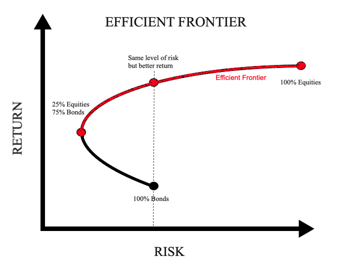
Picture every possible portfolio of your chosen assets on a two‑axis chart:

X‑axis: annualised volatility (risk)
Y‑axis: expected annual return

Most dots live in the middle. The efficient frontier is the upper‑left edge of that cloud — the set of portfolios that deliver the highest return for a given level of risk (or, flipped around, the lowest risk for a chosen return).
If your portfolio sits below that curve, you’re either leaving money on the table or accepting more stress than necessary.

💡 2 The intuition before the equations¶

Diversify: mix assets that don’t move in perfect lock‑step.
Risk–reward trade‑off: extra risk can buy extra return, but not automatically.
Optimise: let math churn through millions of weight combinations and keep only the “best so far”.

That’s the whole trick. No black magic required.

📐 3 A pinch of maths (kept gentle)¶

For a portfolio with weights w, the expected return \( \mu_p \) and volatility \( \sigma_p \) are

\[ \mu_p = \mathbf{w}^\top \boldsymbol{\mu}, \qquad \sigma_p = \sqrt{\mathbf{w}^\top \Sigma \mathbf{w}} \]

where

\( \boldsymbol{\mu} \) — vector of mean asset returns
\( \Sigma \) — covariance matrix of those returns

To trace the frontier we repeatedly solve:

\[ \begin{aligned} \min_{\mathbf{w}}\;& \mathbf{w}^\top \Sigma \mathbf{w} \\ \text{s.t. } & \mathbf{w}^\top \boldsymbol{\mu} \ge \mu_{\text{target}} \\ & \mathbf{1}^\top \mathbf{w} = 1,\; \mathbf{w} \ge 0 \end{aligned} \]

(Here we forbid short‑selling. Remove \( \mathbf{w} \ge 0 \) if you’re fine with shorts.)

🧪 4 Doing it in code (five lines, promise)¶

ef_returns, ef_vols = construct_efficient_frontier(
    returns=my_returns,      # DataFrame of daily % returns
    tickers=my_tickers,
    num_points=100
)

PortfolioPlotter.plot_efficient_frontier(
    port_vols, port_returns, sharpe,
    ef_vols, ef_returns, max_idx
)

construct_efficient_frontier loops over 100 target returns, feeds each optimisation to cvxpy, and stores the resulting risks.
plot_efficient_frontier colours random portfolios by Sharpe ratio so you can spot the sweet spot instantly.

🖼️ 5 How to read the picture¶

Black line: efficient frontier
Red dot: portfolio with the highest Sharpe ratio among the random samples
Sea of dots: random portfolios — most are, frankly, mediocre

Slide leftwards until lowering volatility starts to shave more return than you’re willing to lose. That’s usually your “happy place”.

✅ 6 Quick checklist¶

[ ] Use at least three years of daily data (more is better).
[ ] Annualise returns and volatilities (* 252) consistently.
[ ] Inspect the covariance matrix for weird outliers.
[ ] Decide on constraints (no shorts? max weight per asset?).
[ ] Run the backtest after fixing weights; don’t peek at the future.

📚 Further reading¶

H. Markowitz — Portfolio Selection (1952)
Grinold & Kahn — Active Portfolio Management
Quantocracy blog posts on efficient‑frontier visualisations

(This guide is for educational purposes only — not investment advice.)